Comm
Filters
One of the most important function in this module is the root_raised_cosine_filter() function but to fully understand the root raised cosine filters, we need first to discuss raised cosine filters.
The raised cosine filter, that can be generated in QOSST using the raised_cosine_filter() function, is defined by it’s frequency response
where \(R_S\) is the symbol rate and \(\beta\) a parameter of the filter called the roll-off which is between 0 and 1.
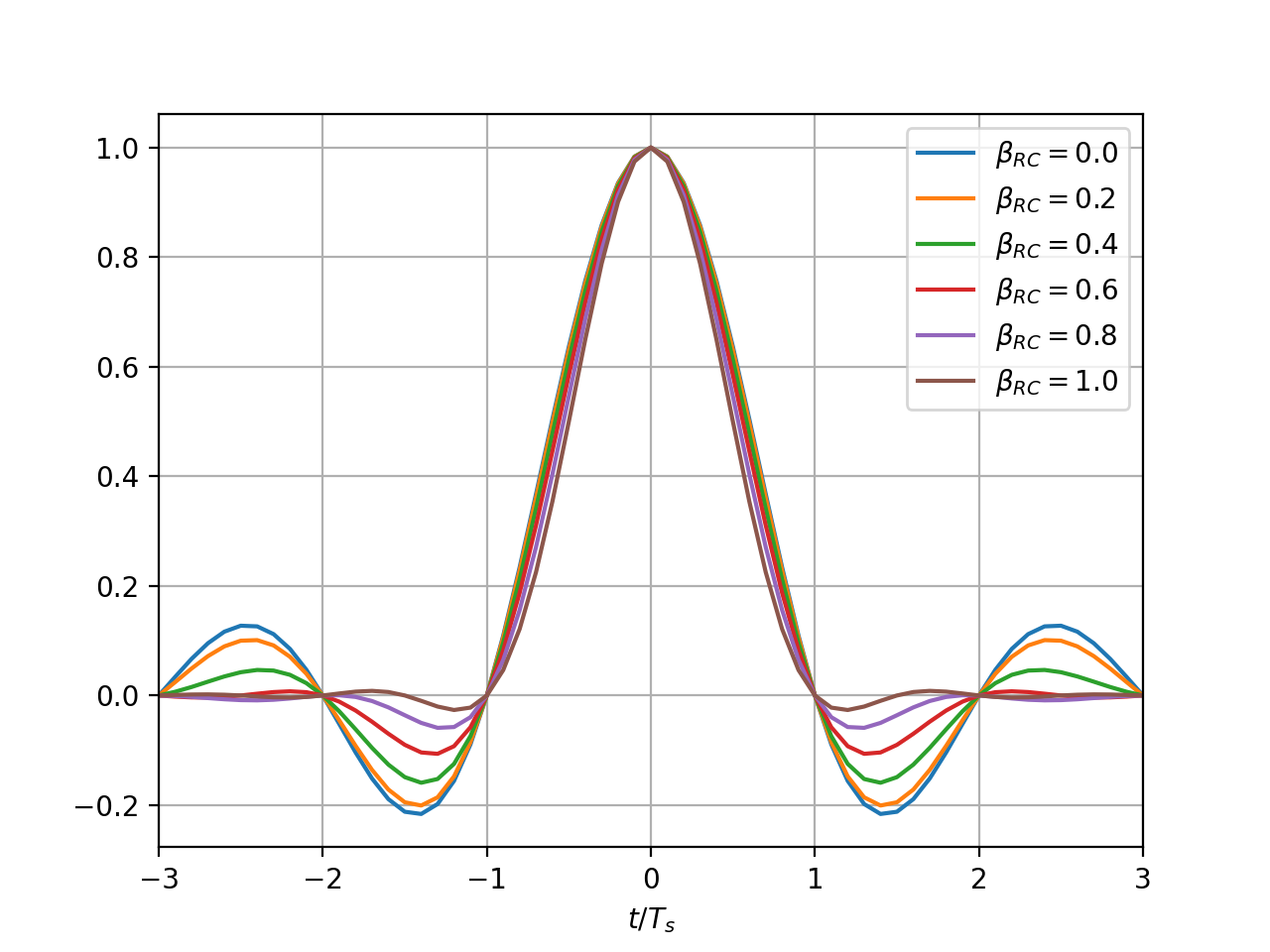
It can be seen that the ase \(\beta=0\) corresponds to a perfect square of bandwidth \(R_S\) in the frequency domain, that will result in a temporal response being a sinc function. Modifying the value of the roll-off will slightly change the form of the sinc in the temporal domain, but leaving the zeros the same place, i.e. for \(t=k\cdot T_S\) with \(k\neq 0\) and \(T_S = 1/R_S\) the symbol period, as can be seen on the following plot:
import matplotlib.pyplot as plt
import numpy as np
from qosst_core.comm.filters import raised_cosine_filter

SAMPLING_RATE = 1e9
SYMBOL_RATE = 100e6
ROLL_OFFS = np.arange(0, 1.01, 0.2)

SPS = int(SAMPLING_RATE / SYMBOL_RATE)
SYMBOL_PERIOD = 1 / SYMBOL_RATE

for beta_rc in ROLL_OFFS:
    times, h_rc = raised_cosine_filter(
        int(10 * SPS), beta_rc, SYMBOL_PERIOD, SAMPLING_RATE
    )
    times_period = times * SYMBOL_RATE

    plt.plot(times_period, h_rc, label=f"$\\beta_{{RC}} = {beta_rc:.1f}$")

plt.grid()
plt.legend()
plt.xlabel("$t / T_s$")
plt.xlim(left=-3, right=3)
plt.show()
(Source code, png, hires.png, pdf)
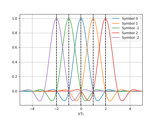
This already hints why the raised cosine filter is very useful: because it minimizes intersymbol interfence. Indeed when performing the convolution, the behaviour in the temporal domain will be that at some \(k\cdot T_S\) for \(k\in\mathbb{Z}\), one symbol will be maximal, and the others 0, as can be seen in the following figure:
import matplotlib.pyplot as plt

from qosst_core.comm.filters import raised_cosine_filter

SAMPLING_RATE = 1e9
SYMBOL_RATE = 100e6
ROLL_OFF = 0.5

N = 3

SPS = int(SAMPLING_RATE / SYMBOL_RATE)
SYMBOL_PERIOD = 1 / SYMBOL_RATE

times, h_rc = raised_cosine_filter(
    int(10 * SPS), ROLL_OFF, SYMBOL_PERIOD, SAMPLING_RATE
)
times_period = times * SYMBOL_RATE

plt.plot(times_period, h_rc, label="Symbol 0")
plt.axvline(0, ls="--", color="black")

for i in range(1, N):
    plt.plot(times_period + i, h_rc, label=f"Symbol {i}")
    plt.plot(times_period - i, h_rc, label=f"Symbol {-i}")
    plt.axvline(i, ls="--", color="black")
    plt.axvline(-i, ls="--", color="black")

plt.grid()
plt.legend()
plt.xlabel("$t / T_s$")
plt.xlim(left=-(N + 2), right=N + 2)
plt.show()
(Source code, png, hires.png, pdf)

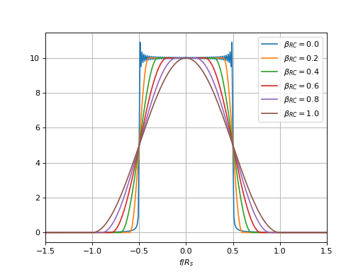
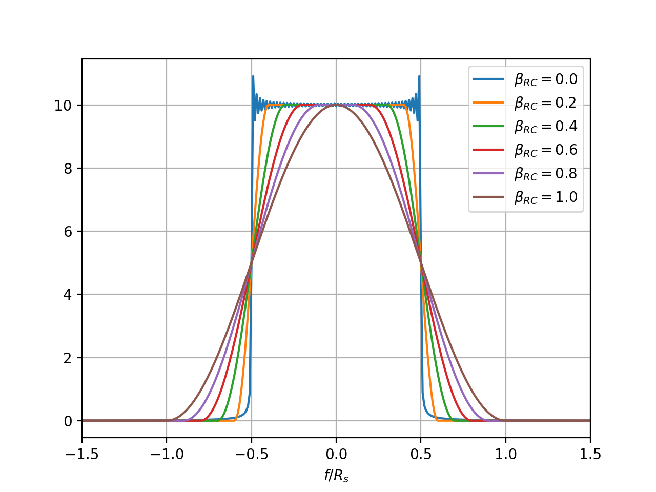
Another advantage of the raised cosine filter is that is frequency response has a finite bandwidth. We already saw that the bandwidth was \(R_S\) when the roll-off was 0, and in the general case, the bandwidth is
As \(R_S\) is at most 1, the bandwidth is between \(R_S\) and \(2\cdot R_S\) as can be seen in the following figure:
import matplotlib.pyplot as plt
import matplotlib.colors as mcolors
import numpy as np
from qosst_core.comm.filters import raised_cosine_filter

SAMPLING_RATE = 1e9
SYMBOL_RATE = 100e6
ROLL_OFFS = np.arange(0, 1.01, 0.2)

SPS = int(SAMPLING_RATE / SYMBOL_RATE)
SYMBOL_PERIOD = 1 / SYMBOL_RATE

COLORS = [color for color in mcolors.TABLEAU_COLORS]

for i, beta_rc in enumerate(ROLL_OFFS):
    times, h_rc = raised_cosine_filter(
        int(100 * SPS), beta_rc, SYMBOL_PERIOD, SAMPLING_RATE
    )
    N = len(h_rc)
    fftfreq = np.fft.fftfreq(N, 1 / SAMPLING_RATE)
    fft = np.fft.fft(h_rc)
    plt.plot(
        fftfreq[: N // 2] / SYMBOL_RATE,
        np.abs(fft)[: N // 2],
        label=f"$\\beta_{{RC}} = {beta_rc:.1f}$",
        color=COLORS[i],
    )
    plt.plot(fftfreq[N // 2 :] / SYMBOL_RATE, np.abs(fft)[N // 2 :], color=COLORS[i])

plt.grid()
plt.legend()
plt.xlabel("$f/R_s$")
plt.xlim(left=-1.5, right=1.5)
plt.show()
(Source code, png, hires.png, pdf)

The effect of the roll-off on the frequency response can also be seen, as it “smoothens” the square. Please note that the frequency response for \(\beta=0\) should be a perfect square but is not due to a finite number of samples (the fft of the filter is plotted, not the formula used in the definition).
For those reasons, the raised cosine is a very strong candidates for the CV-QKD transmissions. However, to reduce the effect of white gaussian noise in the channel, it is usual to apply a matched filter on the receiver side. Hence, it is possible to define a root raised cosine as
and it can be shown that the root raised cosine is its own matched filter, so we can apply a root raised cosine at Alice’s side and a root raised cosine at Bob’s side, that will be in total a raised cosine filter.
Zadoff-Chu sequence
The Zadoff-Chu sequence is a complex sequence defined by
where \(L_{ZC}\) is the length of the sequence and \(R_{ZC}<L_{ZC}\) is the root of the sequence. Moreover, it is imposed that R_{ZC} and L_{ZC} are coprimes, i.e. that \(\text{gcd}(R_{ZC}, L_{ZC}) = 1\). \(c_f\) is defined as \(c_f = L_{ZC} \text{mod} 2\) and \(q\) is the cyclic shift.
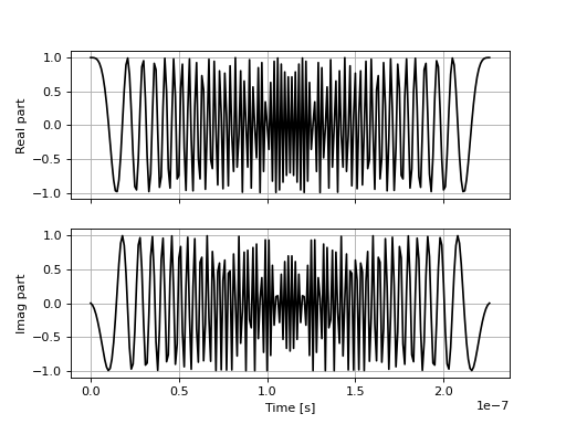
Here is an example of the real and imaginary part of a Zadoff-Chu sequence:
import matplotlib.pyplot as plt
import numpy as np
from qosst_core.comm.zc import zcsequence

SAMPLING_RATE = 1e9
ROOT = 1
LENGTH = 227

sequence = zcsequence(ROOT, LENGTH, cyclic_shift=0)
times = np.arange(len(sequence)) / SAMPLING_RATE

fig, (ax1, ax2) = plt.subplots(2, 1, sharex=True)
ax1.plot(times, sequence.real, color="black")
ax2.plot(times, sequence.imag, color="black")
ax2.set_xlabel("Time [s]")
ax1.set_ylabel("Real part")
ax2.set_ylabel("Imag part")
ax1.grid()
ax2.grid()
plt.show()
(Source code, png, hires.png, pdf)

The Zadoff-Chu sequences are constant modulus and have good auto-correlation properties that results in a good candidates for frame synchronisation.