Modulation

The qosst_core.modulation module offers several format of modulation for CV-QKD:

Gaussian (GaussianModulation);
Phase Shift Keying (PSKModulation);
Quadrature Amplitude Modulation (QAMModulation);
Probabilistic Constellation Shaping Quadrature Amplitude Modulation (PCSQAMModulation);
Binomial Quadrature Amplitude Modulation (BinomialQAM);
Single point modulation (SinglePointModulation).

They can all be used in the CV-QKD software as they respect the same coding formalism and inherits from the qosst_core.modulation.modulation.Modulation class.

In general, the modulation can be used as follows:

from qosst_core.modulation import PSKModulation

modulation = PSKModulation(1, 4) # 1 for the variance, 4 for the size i.e. 4-PSK (or QPSK)
points = modulation.modulate(1000) # Generate 1000 random symbols from this modulation

If you are using the GaussianModulation, the size parameter is unused, and a good behaviour is to put 0.

For an extended documentation on the modulations, check the API documentation.

In the following we present each modulation and an example code, with plot.

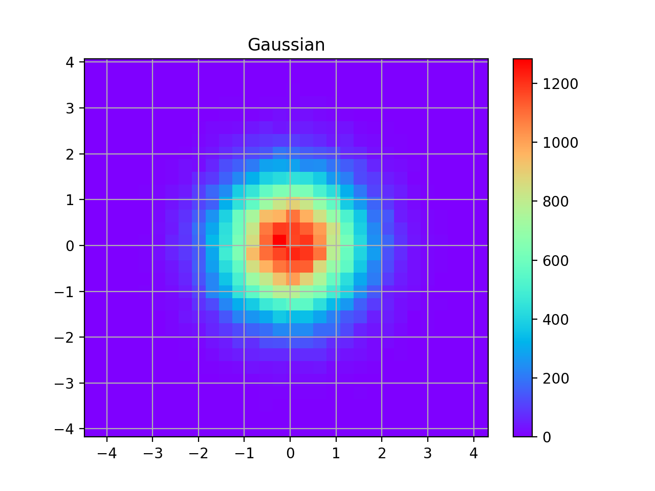
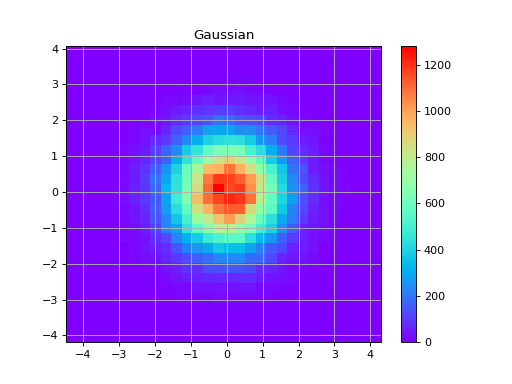
Gaussian

The Gaussian modulation is modulating both quadratures with a Gaussian distribution with same variance (or standard deviation).

Here is a plot of a Gaussian distribution:

import matplotlib.pyplot as plt
import numpy as np

from qosst_core.modulation import GaussianModulation

modulation = GaussianModulation(1)
points = modulation.modulate(100000)
heatmap, xedges, yedges = np.histogram2d(points.real, points.imag, bins=30)
extent = [xedges[0], xedges[-1], yedges[0], yedges[-1]]

plt.imshow(heatmap.T, extent=extent, origin="lower", cmap="rainbow")
plt.title("Gaussian")
plt.colorbar()
plt.grid()
plt.show()

(Source code, png, hires.png, pdf)

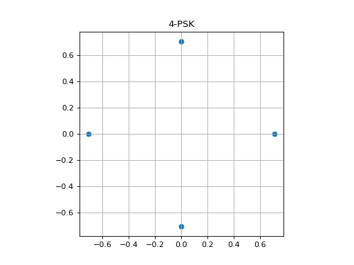
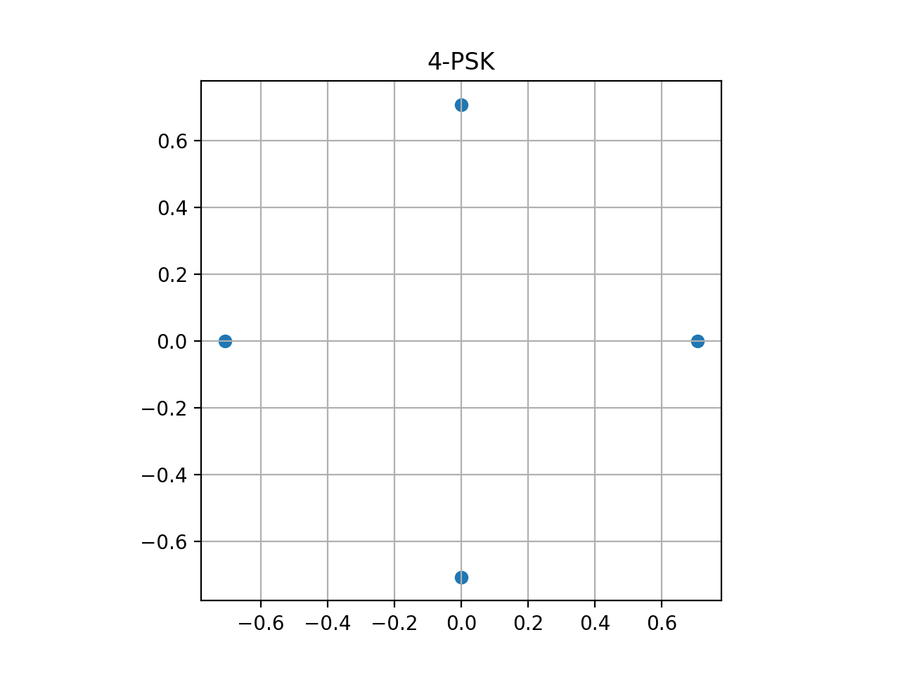
Phase Shift Keying (PSK)

The Phase Shift Keying modulation (PSK) is a modulation with fixed amplitude. It places the points on a circle with a constant angle difference (it also happened to be the unitary roots). For a size \(M\), the set of points is

\[X + j Y = \exp\left(jK\frac{2\pi}{M}\right)\]

with \(K\) following a uniform distribution on \((0, M-1)\)

\[K\sim U(0,M-1)\]

up to a global scaling.

For \(M\) to be a valid size for a \(M\)-PSK, it should be a power of 2 (at least in our context).

We now plot examples of the constellation for \(M\)-PSK (\(M=4\), \(M=8\)) but by plotting the constellation (set of points) directly, and not actually generating data.

4-PSK

from qosst_core.modulation import PSKModulation
import matplotlib.pyplot as plt

modulation = PSKModulation(1, 4)
points = modulation.constellation
plt.scatter(points.real, points.imag)
plt.title("4-PSK")
plt.grid()
plt.gca().set_aspect("equal")
plt.show()

(Source code, png, hires.png, pdf)

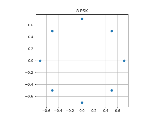
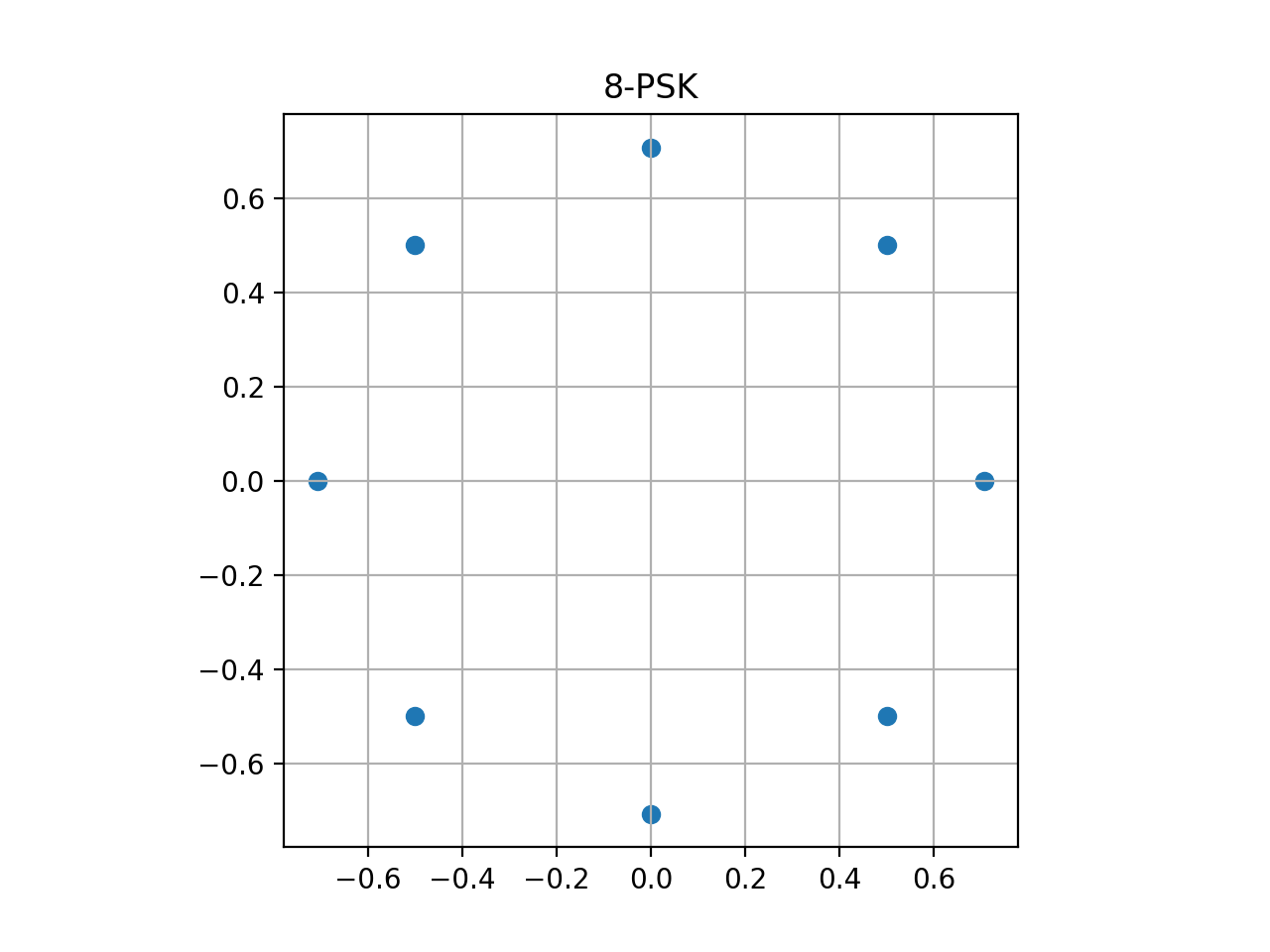
8-PSK

from qosst_core.modulation import PSKModulation
import matplotlib.pyplot as plt

modulation = PSKModulation(1, 8)
points = modulation.constellation
plt.scatter(points.real, points.imag)
plt.title("8-PSK")
plt.grid()
plt.gca().set_aspect("equal")
plt.show()

(Source code, png, hires.png, pdf)

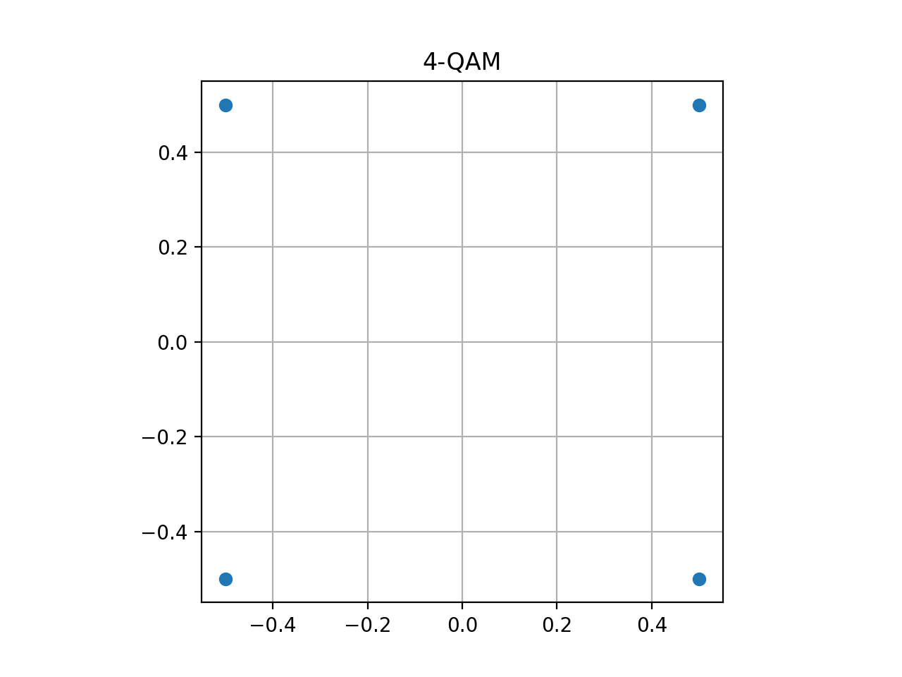
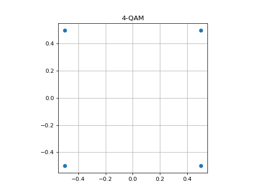
Quadrature Amplitude Modulation (QAM)

The Quadrature Amplitude modulation (QAM) is a modulation displayed on a grid of size \(\sqrt{M}\times\sqrt{M}\). The points are placed uniformly on this grid according to the following distribution:

\[X +jY \sim \left(2\times U\left(-\frac{\sqrt{M}}{2}, \frac{\sqrt{M}}{2} -1\right)+1\right) + j\left(2\times U\left(-\frac{\sqrt{M}}{2}, \frac{\sqrt{M}}{2} -1\right) + 1\right)\]

where \(U\) is once again the uniform distribution and up to a global scaling.

For \(M\) to be a valid size for a \(M\)-QAM, it should be a power of 2 and a square, meaning that \(\sqrt{M}\) should be an integer (at least in our context).

We now plot examples of the constellation for \(M\)-QAM (\(M=4\), \(M=16\) and \(M=256\)) but by plotting the constellation (set of points) directly, and not actually generating data.

4-QAM

from qosst_core.modulation import QAMModulation
import matplotlib.pyplot as plt

modulation = QAMModulation(1, 4)
points = modulation.constellation
plt.scatter(points.real, points.imag)
plt.title("4-QAM")
plt.grid()
plt.gca().set_aspect("equal")
plt.show()

(Source code, png, hires.png, pdf)

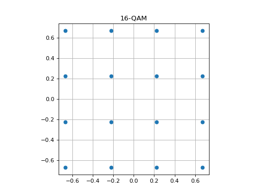
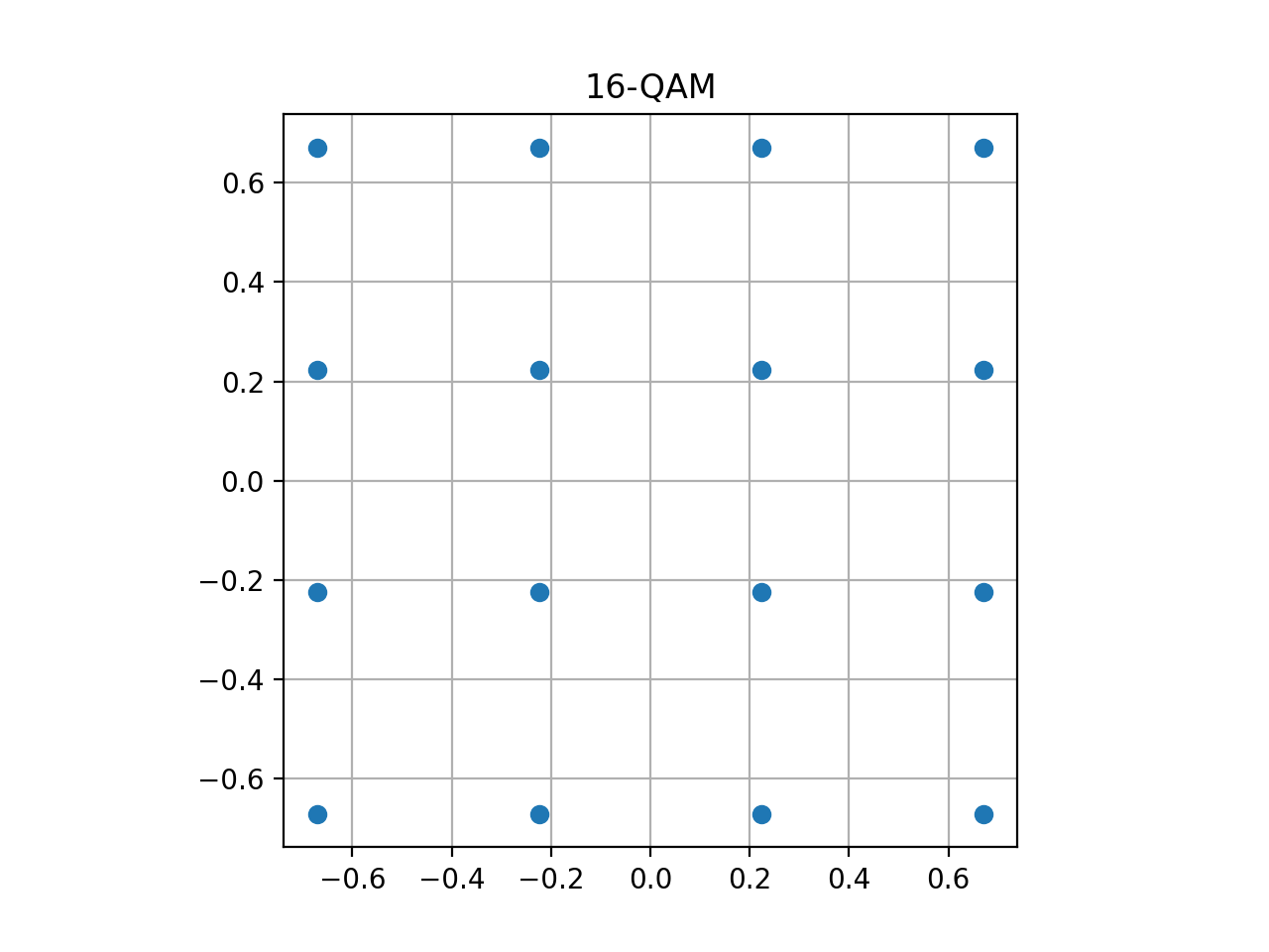
16-QAM

from qosst_core.modulation import QAMModulation
import matplotlib.pyplot as plt

modulation = QAMModulation(1, 16)
points = modulation.constellation
plt.scatter(points.real, points.imag)
plt.title("16-QAM")
plt.grid()
plt.gca().set_aspect("equal")
plt.show()

(Source code, png, hires.png, pdf)

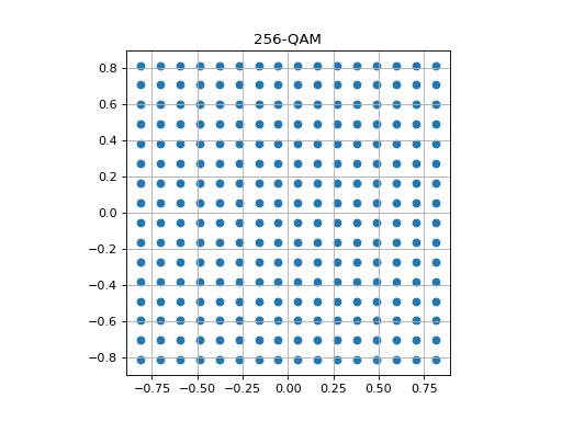
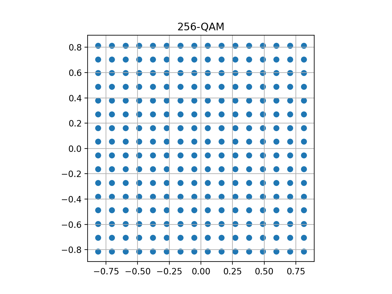
256-QAM

from qosst_core.modulation import QAMModulation
import matplotlib.pyplot as plt

modulation = QAMModulation(1, 256)
points = modulation.constellation
plt.scatter(points.real, points.imag)
plt.title("256-QAM")
plt.grid()
plt.gca().set_aspect("equal")
plt.show()

(Source code, png, hires.png, pdf)

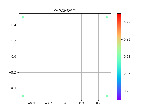
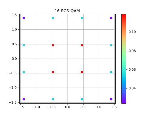
Probabilistic Constellation Shaping QAM (PCS-QAM)

The Probabilistic Constellation Shaping Quadrature Amplitude Modulation (PCS-QAM) is a modulation where the constellation is the same as the QAM, but this time the point are not chosen uniformly on the grid, but are chosen to approximate Gaussian.

A way to define it it to say that for each point \((x,y)\) on the QAM lattice, the probability of the point to be chosen is

\[p(x,y) \propto \exp(-\nu(x^2+y^2))\]

where \(\nu\) is a parameter related to the variance, and up to a global scale.

For \(M\) to be a valid size for a \(M\)-PCSQAM, it should be a power of 2 and a square, meaning that \(\sqrt{M}\) should be an integer (at least in our context).

In the following we plot examples for \(M=4\), \(M=16\) and \(M=256\).

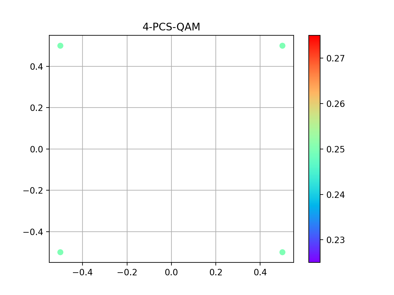
4-PCS-QAM

import matplotlib.pyplot as plt

from qosst_core.modulation import PCSQAMModulation

modulation = PCSQAMModulation(1, 4, 0.1)
points = modulation.constellation
colors = modulation.distribution
plt.scatter(points.real, points.imag, c=colors, cmap="rainbow")
plt.title("4-PCS-QAM")
plt.colorbar()
plt.grid()
plt.show()

(Source code, png, hires.png, pdf)

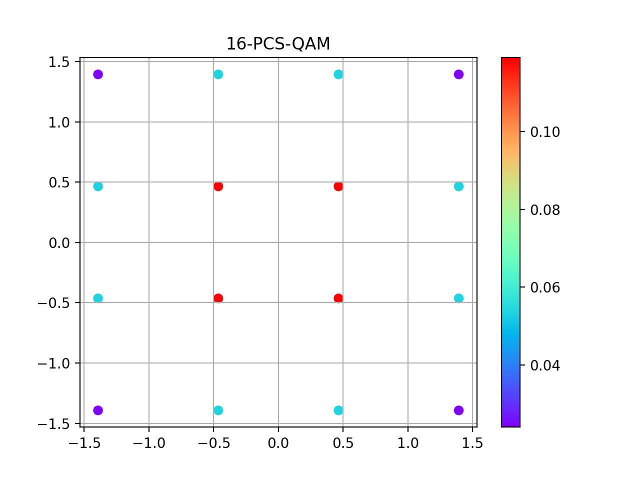
16-PCS-QAM

import matplotlib.pyplot as plt

from qosst_core.modulation import PCSQAMModulation

modulation = PCSQAMModulation(3, 16, nu=0.1)
points = modulation.constellation
colors = modulation.distribution
plt.scatter(points.real, points.imag, c=colors, cmap="rainbow")
plt.title("16-PCS-QAM")
plt.colorbar()
plt.grid()
plt.show()

(Source code, png, hires.png, pdf)

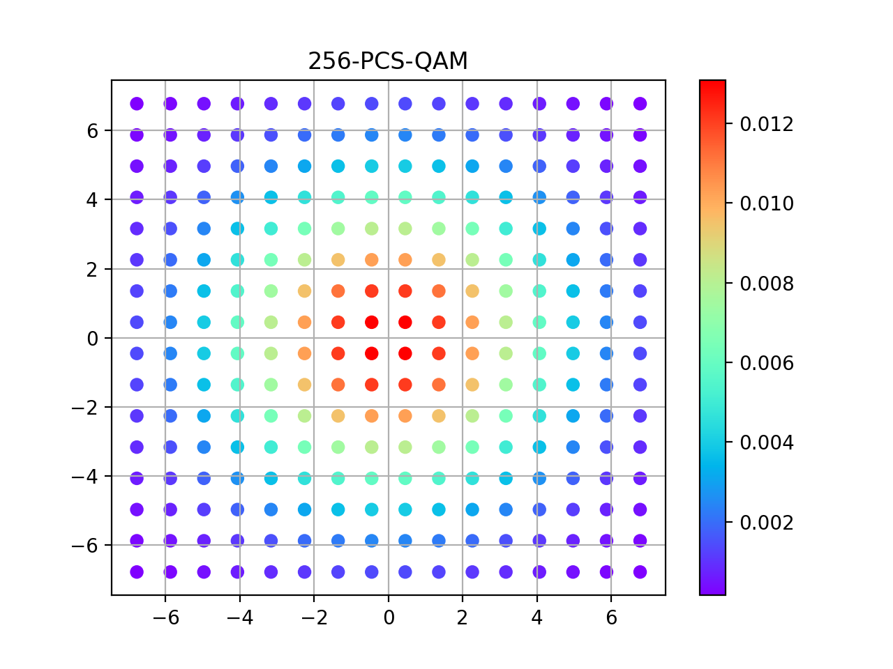
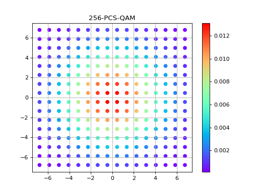
256-PCS-QAM

import matplotlib.pyplot as plt

from qosst_core.modulation import PCSQAMModulation

modulation = PCSQAMModulation(35, 256, nu=0.01)
points = modulation.constellation
colors = modulation.distribution
plt.scatter(points.real, points.imag, c=colors, cmap="rainbow")
plt.title("256-PCS-QAM")
plt.colorbar()
plt.grid()
plt.show()

(Source code, png, hires.png, pdf)

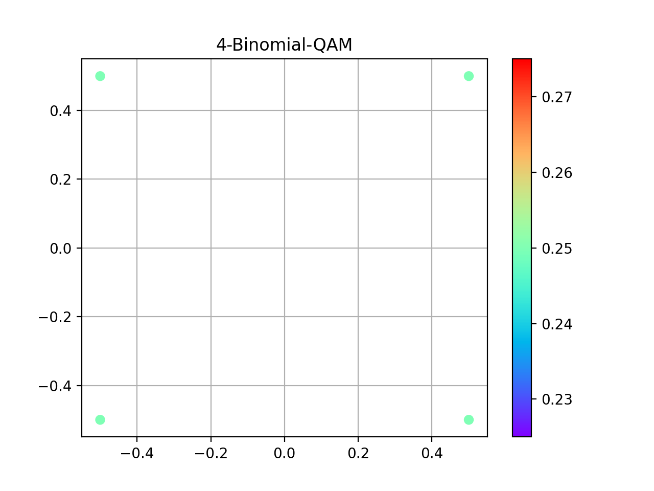
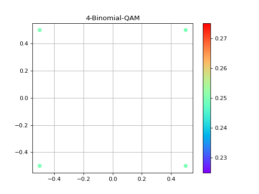
Binomial Quadrature Amplitude Modulation (Binomial QAM)

4-BINOMIAL-QAM

import matplotlib.pyplot as plt

from qosst_core.modulation import BinomialQAMModulation

modulation = BinomialQAMModulation(1, 4)
points = modulation.constellation
colors = modulation.distribution
plt.scatter(points.real, points.imag, c=colors, cmap="rainbow")
plt.title("4-Binomial-QAM")
plt.colorbar()
plt.grid()
plt.show()

(Source code, png, hires.png, pdf)

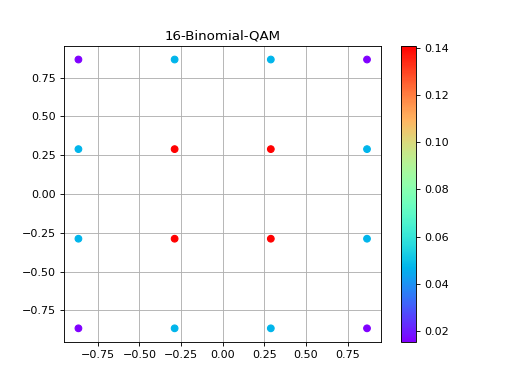
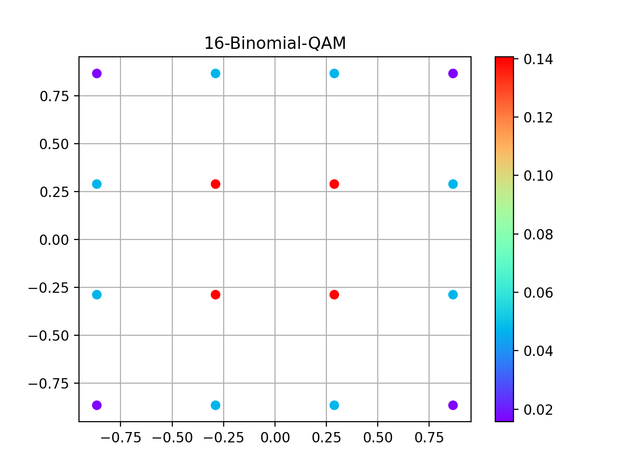
16-BINOMIAL-QAM

import matplotlib.pyplot as plt

from qosst_core.modulation import BinomialQAMModulation

modulation = BinomialQAMModulation(1, 16)
points = modulation.constellation
colors = modulation.distribution
plt.scatter(points.real, points.imag, c=colors, cmap="rainbow")
plt.title("16-Binomial-QAM")
plt.colorbar()
plt.grid()
plt.show()

(Source code, png, hires.png, pdf)

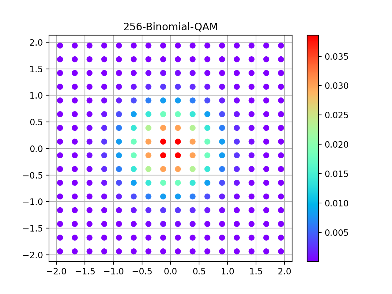
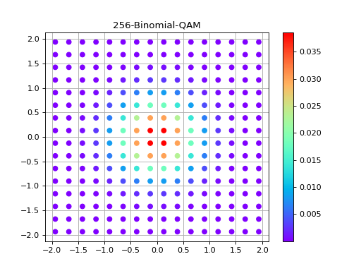
256-BINOMIAL-QAM

import matplotlib.pyplot as plt

from qosst_core.modulation import BinomialQAMModulation

modulation = BinomialQAMModulation(1, 256)
points = modulation.constellation
colors = modulation.distribution
plt.scatter(points.real, points.imag, c=colors, cmap="rainbow")
plt.title("256-Binomial-QAM")
plt.colorbar()
plt.grid()
plt.show()

(Source code, png, hires.png, pdf)

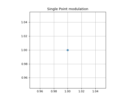
Single point

The single point modulation is just a single point and just should be used for test purposes.

Here is an example with the point \((1,1)\).

from qosst_core.modulation import SinglePointModulation
import matplotlib.pyplot as plt

modulation = SinglePointModulation(x=1, y=1)
points = modulation.modulate(1)
plt.scatter(points.real, points.imag)
plt.title("Single Point modulation")
plt.grid()
plt.gca().set_aspect("equal")
plt.show()

(Source code, png, hires.png, pdf)